At Simpson Strong-Tie, we do our best to offer tools that make your job easier. One such tool is the Screw Substitution Calculator. It’s a quick and easy-to-use web app created to help you calculate and design using Simpson Strong-Tie fasteners. The app can be used in two ways: (1) to design for a given load and (2) to provide a substitution for NDS fasteners. The app covers design for withdrawal loading, lateral loading and multi-ply connections. For each of these applications you can either design for a load or input the specified NDS fasteners and design an alternate Simpson Strong-Tie screw substitution. The app can generate detailed calculations in a PDF format for any of the selections made, and these calculations can be used for submittals.
Note that although the tool currently does not address corrosion issues, corrosion resistance should be an important consideration before selecting screws for your application.
Below is a screenshot of the Screw Substitution Calculator. As explained above, the app can design for
- Withdrawal Loading
- Lateral Loading
- Multi-Ply Connections

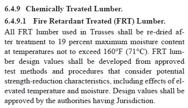
The input sections for Withdrawal Loading and Lateral Loading (parallel or perpendicular to grain) are similar. A screenshot of Lateral Load Parallel to Grain is shown below.
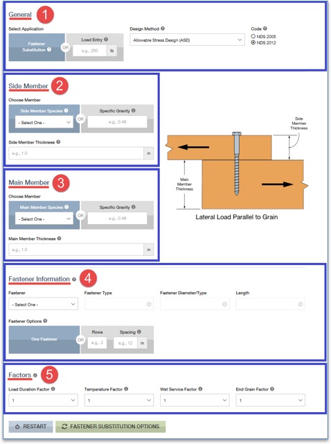
Step 1: General Information – In this section, you are requested to select either Fastener Substitution or a Load Entry. If you choose fastener substitution, the app will request in step 4, Fastener Information, that you enter the original fastener design. The fastener substitution calculator will provide Simpson Strong-Tie fastener alternatives for the NDS fasteners. The NDS fasteners covered in this app are bolts, lag screws, wood screws and nails.
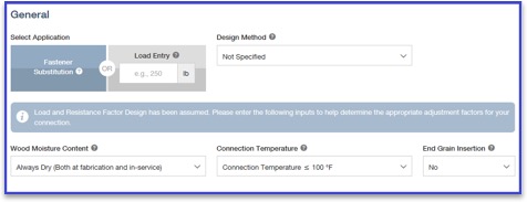
If you choose Load Entry, you will notice that the Fastener Information step will disappear and no longer be available for input. Next, select a category from the Design Method section. Available options are Allowable Stress Design (ASD), Load and Resistance Factor Design (LRFD) and Not Specified, if you are not sure of the design method. If the Not Specified option is selected, the design assumes the Load and Resistance Factor Design method, and it further prompts you to answer a few more questions related to Wood Moisture Content, Connection Temperature and End Grain Insertion.
Step 2: Side Member – In this section, all the information regarding the side member is entered. You can either select a species from the drop-down list or enter the specific gravity of the member manually in the text box. The information button lists all the available specific gravities for wood species combinations from NDS. Then enter the (actual, not nominal) thickness of the side member.
Step 3: Main Member – Similar to step 2, enter all information regarding the main member.
Step 4: Fastener Information – If the Fastener Substitution option is selected in step 1, step 4 will require you to enter information about the NDS fasteners used in the initial design. Enter the fastener type (bolt, lag screw, screw or nail), along with its diameter and length. From the fastener option list you can either select one fastener substitute at a time for each NDS fastener or enter the number of rows and the spacing of NDS-designed fasteners to determine Simpson Strong-Tie fastener options and their spacing requirements.
Step 5: Factors – Enter all factors required for designing the connection. Information pertaining to each factor is provided by clicking the information (i) button. You can use this as a guide for entering the factors.
Once all the input is entered, click on the FASTENER SUBSTITUTION OPTIONS button.

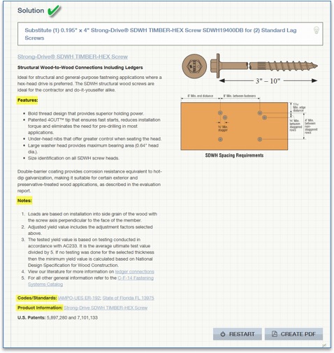
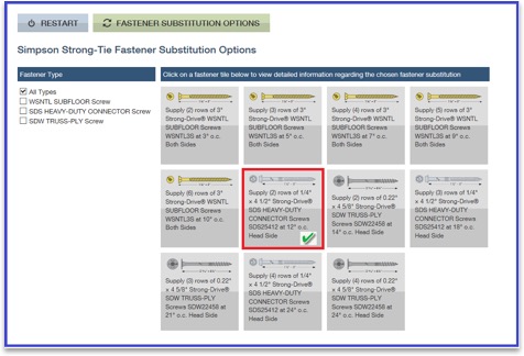
Clicking FASTENER SUBSTITUTION OPTIONS reveals the available solutions. As a default, the All Types box is checked under Fastener Type, as shown above. You can refine the solutions by unchecking this box and selecting any of the specific fasteners listed – SDWH TIMBER-HEX Screw solutions, for example. On the right, the available solutions are displayed for selection. When a selection is made, the app displays all the input and output for that solution as shown in the screenshot below. You can also create a PDF copy for any of the solutions by clicking on CREATE PDF button.


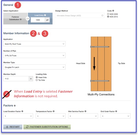
For Multi-Ply Connections, the input for side members and main members is combined into Member Information as shown in the screenshot below. Once the input is entered, click the FASTENER SUBSTITUTION OPTIONS button to display results. Similar to withdrawal loading or lateral loading, you can create a PDF copy of the calculations.
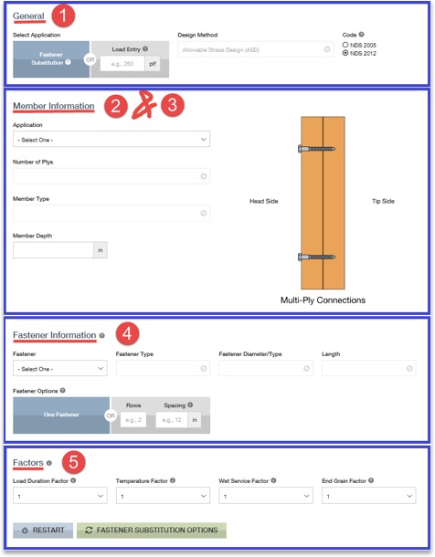
Let’s design a 3-ply connection with (3) 2 x 12 DF members for a load of 1,000 plf.
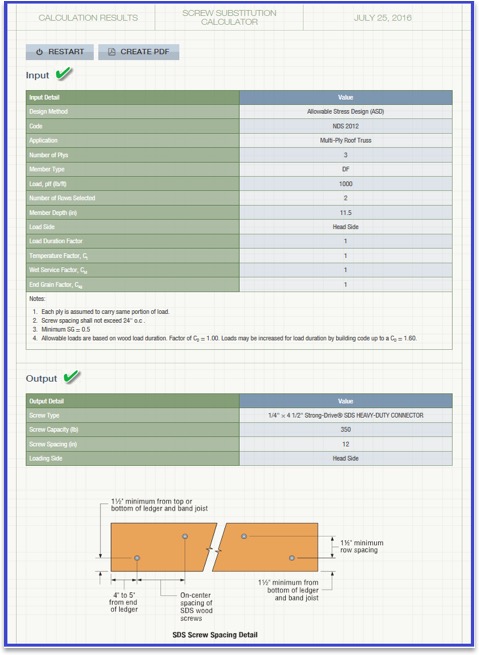
By clicking FASTENER SUBSTITUTION OPTIONS, you can see all the available Simpson Strong-Tie fastener solutions. You can then select any of the options to generate detailed output. A screenshot of the output, solution and information regarding the selected fastener is displayed below. You can create a PDF copy of the solution by clicking the CREATE PDF button.

Now that you know how easy it is to design using our Screw Substitution Calculator, you can start using this tool for your future projects. We welcome your feedback on the features you find useful as well as on how we could make this program better suit your needs. Let us know in the comments below.


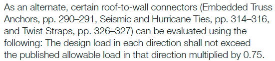


 There are products used in every building not referenced by the codes or standards.
 limitations.