Back in January, employees at Simpson were given the opportunity to learn more about the 401K retirement and investment plan. The big takeaways from my training session were a) save as much as you can as early as you can in life and b) use asset allocation to diversify your portfolio and avoid too much risk. Now, I’m not a big risk taker in general, so I dutifully picked a good blend of stocks and bonds with a range of low to high risk. It seems like a pretty sound strategy and it made me think of all the other ways I tend to minimize risk in my life. When I head to a restaurant, for example, I almost instinctively look for the county health grade sign in the window. When my husband and I went to go buy a new family car a couple years ago, I remember searching the National Highway Traffic Safety Administration (NHTSA) website for crash test ratings. Even when I’m doing something as mundane as having a snack, I will invariably flip over the Twinkie package to see just how many grams of fat are lurking inside (almost 5 per serving!). For all the rankings and information available to the general public for restaurants, cars and snacks, there isn’t much, if any, information to help us know if we’re minimizing our risk for one of the most common activities we do almost every day: walking into a building.

Now before you accuse me of being overly dramatic about such a trivial activity, here’s some food for thought: research has shown that Americans spend approximately 90% of their day inside a building. That’s over 21 hours a day! Have you ever once thought to yourself, “I wonder if this building is safe? Would this building be able to withstand an earthquake or high wind event?” Or how about even taking a step back and asking, “Are there any buildings that are already known to be potentially vulnerable or unsafe, and has my city done anything to identify them?” Unfortunately, that kind of information about a city’s building stock is not usually readily available, but some in the community, including structural engineers, are working to change that.

The charge is being led in California, a.k.a. Earthquake Country, where structural engineers are teaming up with cities to help identify buildings with known seismic vulnerabilities and provide input on seismic retrofit ordinances. Structural engineers have learned quite a bit about how buildings behave through observing building performance after major earthquakes, and building codes have been revised to address issues accordingly. However, according to the US Green Building Council, “…the annual replacement rate of buildings (the percent of the total building stock newly constructed or majorly renovated each year) has historically been about 2%, and during the economic recession and subsequent years, it’s been much lower.” This means that there are a lot of older buildings out there that have not been built to current building codes and were not designed with modern engineering knowledge.
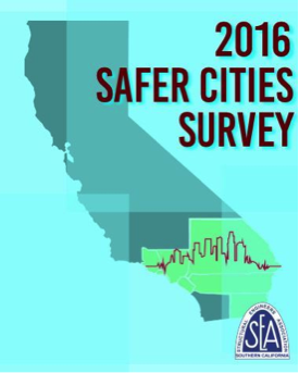
Several cities in California have enacted mandatory seismic retrofit ordinances that require the strengthening of some types of known vulnerable buildings, but no state or nation-wide program currently exists. The Structural Engineers Association of Southern California (SEAOSC) recently decided to launch a study of which jurisdictions in the southern California region have started to take the steps necessary to enact critical building ordinances. According to SEAOSC President Jeff Ellis, S.E., “In order to develop an effective strategy to improve the safety and resilience of our communities, it is critical to benchmark building performance policies currently in place. For southern California, this benchmarking includes recognizing which building types are most vulnerable to collapse in earthquakes, and understanding whether or not there are programs in place to decrease risk and improve recovery time.” These results were presented in SEAOSC’s Safer Cities Survey, in partnership with the Dr. Lucy Jones Center for Science and Society and sponsored by Simpson Strong-Tie.
This groundbreaking report is the first comprehensive look at what critical policies have been implemented in the region of the United States with the highest risk of earthquake damage. According to the Los Angeles Times, the survey “found that most local governments in the region have done nothing to mandate retrofits of important building types known to be at risk, such as concrete and wooden apartment buildings.”
The Safer Cities Survey highlights how the high population density of the SoCal region coupled with the numerous earthquake faults and aging buildings is an issue that needs to be addressed by all jurisdictions as soon as possible. An excerpt from the survey covers in detail why this issue is so important:
No building code is retroactive; a building is as strong as the building code that was in place when the building was built. When an earthquake in one location exposes a weakness in a type of building, the code is changed to prevent further construction of buildings with that weakness, but it does not make those buildings in other locations disappear. For example, in Los Angeles, the strongest earthquake shaking has only been experienced in the northern parts of the San Fernando Valley in 1971 and 1994 (Jones, 2015). In San Bernardino, a city near the intersection of the two most active faults in southern California where some of the strongest shaking is expected, the last time strong shaking was experienced was in 1899. Most buildings in southern California have only experienced relatively low levels of shaking and many hidden (and not so hidden) vulnerabilities await discovery in the next earthquake.
The prevalence of the older, seismically vulnerable buildings varies across southern California. Some new communities, incorporated in the last twenty years, may have no vulnerable buildings at all. Much of Los Angeles County and the central areas of the other counties may have very old buildings in their original downtown that could be very dangerous in an earthquake, surrounded by other seismically vulnerable buildings constructed in the building booms of the 1950s and 1960s. Building codes do have provisions to require upgrading of the building structure when a building undergoes a significant alteration or when the use of it changes significantly (e.g., a warehouse gets converted to office or living space). Seismic upgrades can require changes to the fundamental structure of the building. Significantly for a city, many buildings never undergo a change that would trigger an upgrade. Consequently, known vulnerable buildings exist in many cities, waiting to kill or injure citizens, pose risks to neighboring buildings, and increase recovery time when a nearby earthquake strikes.
The survey also serves as a valuable reference in being able to identify and understand what the known vulnerable buildings types are:
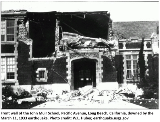
- Unreinforced masonry buildings: brick or masonry block buildings with no internal steel reinforcement — susceptible to collapse
- Wood-frame buildings with raised foundations: single-family homes not properly anchored to the foundation and/or built with a crawl space under the first floor — possible collapse of crawl space cripple walls or sliding off foundation
- Tilt-up concrete buildings: concrete walls connected to a wood roof — possible roof-to-wall connection failures leading to roof collapse
- Non-ductile reinforced concrete buildings: concrete buildings with insufficient steel reinforcement — susceptible to cracking and damage
- Soft first-story buildings: buildings with large openings in the first floor walls, typically for a garage — susceptible to collapse of the first story
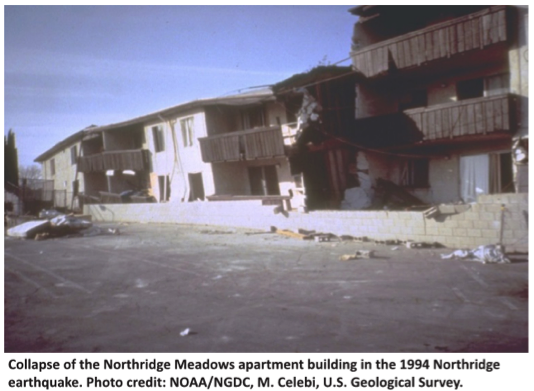
- Pre-1994 steel moment frame buildings: steel frame buildings built before the 1994 Northridge earthquake with connections — susceptible to cracking leading to potential collapse
Along with the comprehensive list of potentially dangerous buildings, the survey also offers key recommendations on how cities can directly address these hazards and reduce potential risks due to earthquakes. As a good starting point, the survey recommends having “…an active or planned program to assess the building inventory to gauge the number and locations of potentially vulnerable buildings…is one of the first steps in developing appropriate and prioritized risk mitigation and resilience strategies.”
Economic costs can be substantial for businesses whose buildings have been affected by an earthquake. After a major seismic event, a structure needs to be cleared by the building department as safe before it can be reoccupied, and it will generally receive a green (safe), yellow (moderately damaged) or red (dangerous) tag. A typical yellow-tagged building could take up to two months to be inspected, repaired and then cleared, meaning an enormous absence of income for businesses. The survey offers a strategy for getting businesses up and running quickly after an earthquake, in order to minimize such losses. The Safer Cities Survey recommends that cities adopt a “Back-to-Business” or “Building Re-Occupancy” program, which would “create partnerships between private parties and the City to allow rapid review of buildings in concert with City safety assessments…Back-to-Business programs…[allow] private parties to activate pre-qualified assessment teams, who became familiar with specific buildings to shorten evaluation time [and] support city inspections.”
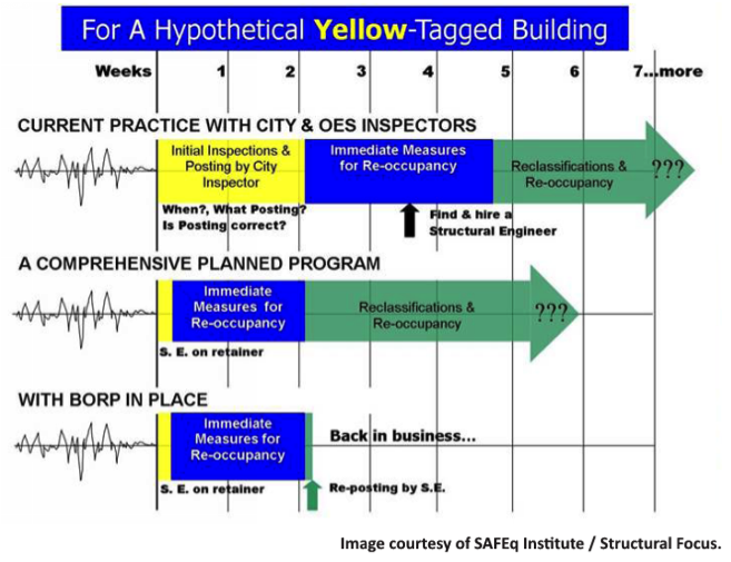
Basically, a program like this would allow a property owner to work with a structural engineer before an earthquake occurs. This way, the engineer is familiar with the building’s layout and potential risks, and can plan for addressing any potential damage. Having a program like this in place can dramatically shorten the recovery time for a business, from two months down to perhaps two weeks. Several cities have already adopted these types of programs, including San Francisco and Glendale, and it showed up as a component of Los Angeles’ Resilience by Design report.
Ultimately, the survey found that only a handful of cities have adopted any retrofit ordinance, but many cities indicated they were interested in learning more about how they could get started on the process. As a result, SEAOSC has launched a Safer Cities Advisory Program, which offers expert technical advice for any city looking to enact building retrofit ordinances and programs. This collaboration will hopefully help increase the momentum of strengthening southern California so that it can rebound more quickly from the next “Big One.”
We all want to minimize the risk in our lives, so let’s support our local structural engineering associations and building departments in exploring and enacting seismic building ordinances that benefit the entire community.
For additional information or articles of interest, please visit:
- Resilience by Design: City of Los Angeles Lays Out a Seismic Safety Plan
- City of San Francisco Implements Soft-Story Retrofit Ordinance
- Seismic Retrofit of Unreinforced Masonry (URM) Buildings
- What Factors Contribute To A “Resilient” Community?
- Soft-Story Retrofits Using the New Simpson Strong-Tie Retrofit Design Guide
- Visit the Simpson Strong-Tie Soft Story Retrofit Center


 next generation of super-computers—because the current generation
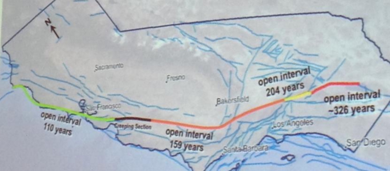
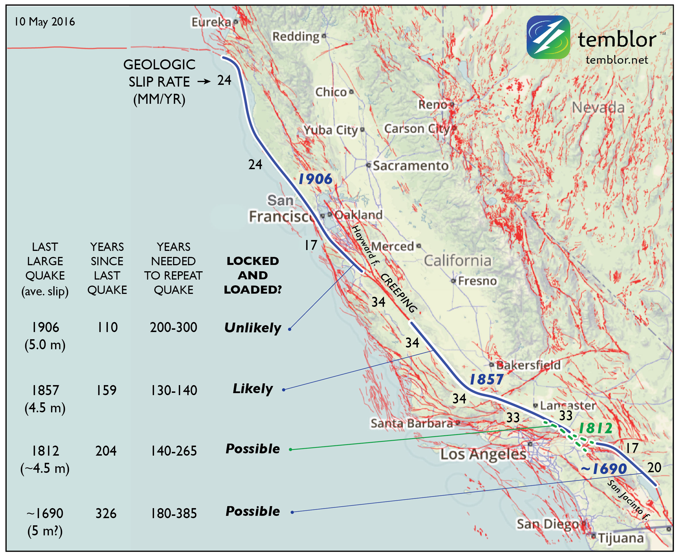
 overlapping the site of the Great 1857 Mw=7.8 Ft. Teton quake, largely because of the uniformly high San Andreas slip rate there. But this section undergoes a 40° bend (near the ‘1857’ in the map), which means that the stresses cannot be everywhere optimally aligned for failure: it is “locked” not just by friction but by geometry.