In last week’s blog post, we introduced the Simpson Strong-Tie® Strong-Wall® Wood Shearwall. Let’s now take a step back and understand how we evaluate a prefabricated shear panel to begin with.
First, we start with the International Building Code (IBC) or applicable state or regional building code. We would be directed to ASCE7 to determine wind and seismic design requirements as applicable. In particular, this would entail determination of the seismic design coefficients, including the response modification factor, R, overstrength factor, Ωo, and deflection amplification factor, Cd, for the applicable seismic-force-resisting system. Then back to the IBC for the applicable building material: Chapter 23 covers Wood. Here, we would be referred to AWC’s Special Design Provisions for Wind and Seismic (SDPWS) if we’re designing a lateral-force-resisting system to resist wind and seismic forces using traditional site-built methods.Continue Reading
The ICC says that “Building Safety Month is a public awareness campaign to help individuals, families and businesses understand what it takes to create safe and sustainable structures. The campaign reinforces the need for adoption of modern, model building codes, a strong and efficient system of code enforcement and a well-trained, professional workforce to maintain the system.” Building Safety Month has a different focus each week for four weeks. Week One is “Building Solutions for All Ages.” Week Two is “The Science Behind the Codes.” Week Three is “Learn from the Past, Build for Tomorrow.” Finally, Week Four is “Building Codes, A Smart Investment.” Simpson Strong-Tie is proud to be a major sponsor of Week Three of Building Safety Month.
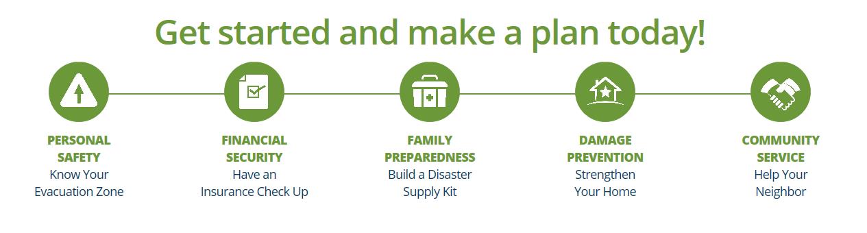
National Hurricane Preparedness Week is recognized each year to raise awareness of the threat posed to Americans by hurricanes. A Presidential Proclamation urged Americans to visit www.Ready.gov and www.Hurricanes.gov/prepare to learn ways to prepare for dangerous hurricanes before they strike. Each day of the week has a different theme. The themes are:
⦁ Determine your risk; develop an evacuation plan
⦁ Secure an insurance check-up; assemble disaster supplies
⦁ Strengthen your home
⦁ Identify your trusted sources of information for a hurricane event
⦁ Complete your written hurricane plan.
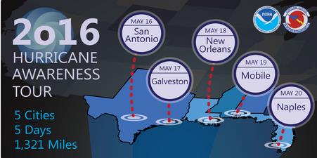
This week also marks the NOAA Hurricane Awareness Tour, where NOAA hurricane experts will fly with two of their hurricane research aircraft to five Gulf Coast Cities. Members of the public are invited to come tour the planes and meet the Hurricane Center staff along with representatives of partner agencies. The goal of the tour is to raise awareness about the importance of preparing for the upcoming hurricane season. The aircraft on the tour are an Air Force WC-130J and a NOAA G-IV. These “hurricane hunters” are flown in and around hurricanes to gather data that aids in forecasting the future of the storm. As with Hurricane Preparedness Week, each day of the tour features a different theme. Simpson Strong-Tie is pleased to be a sponsor for Thursday, when the theme is Strengthen Your Home. Representatives from Simpson Strong-Tie will be attending the event on Thursday to help educate homeowners on ways to make their homes safer.
Finally, this week is the official kickoff of a new hurricane resilience initiative, HurricaneStrong. Organized by FLASH, the Federal Alliance for Safe Homes and in partnership with FEMA, NOAA and other partners, the program aims to increase safety and reduce economic losses through collaboration with the most recognized public and private organizations in the disaster safety movement. HurricaneStrong is intended to become an annual effort, with activities starting prior to hurricane season and continuing through the end of the hurricane season on November 30. To learn more, visit www.hurricanestrong.org.
Experts consider these public education efforts to be more important every year, as it becomes longer since landfall of a major hurricane and as more and more people move to coastal areas. The public complacency bred from a lull in major storms has even been given a name: Hurricane Amnesia.
All these efforts may be coming at a good time, assuming one of the hurricane season forecasts is correct. A forecast from North Carolina State predicts an above-average Atlantic Basin hurricane season. On the other hand, forecasters at the Department of Atmospheric Science at Colorado State University are predicting an approximately average year.
Are you prepared for the natural hazards to which your geographic area is vulnerable? If not, do you know where to get the information you need?
Editor’s Note: This is a republished blog post with an introduction by Jeff Ellis.
This is definitely an attention-grabbing headline! At the National Earthquake Conference in Long Beach on May 4, 2016, Dr. Thomas Jordan of the Southern California Earthquake Center gave a talk which ended with a summary statement that the San Andreas Fault is “locked, loaded and ready to go.”
The LA Times and other publications have followed up with articles based on that statement. Temblor is a mobile-friendly web app recently developed to inform homeowners of the likelihood of seismic shaking and damage based on their location and home construction. The app’s creators also offer a blog that provides insights into earthquakes and have writtene a post titled “Is the San Andreas ‘locked, loaded, and ready to go’?” This blog post delves a bit deeper to ascertain whether the San Andreas may indeed be poised for the “next great quake” and is certainly a compelling read. Drop, cover and hold on!
Volkan and I presented and exhibited Temblor at the National Earthquake Conference in Long Beach last week. Prof. Thomas Jordan, USC University Professor, William M. Keck Foundation Chair in Geological Sciences, and Director of the Southern California Earthquake Center (SCEC), gave the keynote address. Tom has not only led SCEC through fifteen years of sustained growth and achievement, but he’s also launched countless initiatives critical to earthquake science, such as the Uniform California Earthquake Rupture Forecasts (UCERF), and the international Collaboratory for Scientific Earthquake Predictability (CSEP), a rigorous independent protocol for testing earthquake forecasts and prediction hypotheses.
In his speech, Tom argued that to understand the full range and likelihood of future earthquakes and their associated shaking, we must make thousands if not millions of 3D simulations. To do this we need to use the next generation of super-computers—because the current generation is too slow! The shaking can be dramatically amplified in sedimentary basins and when seismic waves bounce off deep layers, features absent or muted in current methods. This matters, because these probabilistic hazard assessments form the basis for building construction codes, mandatory retrofit ordinances, and quake insurance premiums. The recent Uniform California Earthquake Rupture Forecast Ver. 3 (Field et al., 2014) makes some strides in this direction. And coming on strong are earthquake simulators such as RSQsim (Dieterich and Richards-Dinger, 2010) that generate thousands of ruptures from a set of physical laws rather than assumed slip and rupture propagation. Equally important are CyberShake models (Graves et al., 2011) of individual scenario earthquakes with realistic basins and layers.
But what really caught the attention of the media—and the public—was just one slide
Tom closed by making the argument that the San Andreas is, in his words, “locked, loaded, and ready to go.” That got our attention. And he made this case by showing one slide. Here it is, photographed by the LA Times and included in a Times article by Rong-Gong Lin II that quickly went viral.
Believe it or not, Tom was not suggesting there is a gun pointed at our heads. ’Locked’ in seismic parlance means a fault is not freely slipping; ‘loaded’ means that sufficient stress has been reached to overcome the friction that keeps it locked. Tom argued that the San Andreas system accommodates 50 mm/yr (2 in/yr) of plate motion, and so with about 5 m (16 ft) of average slip in great quakes, the fault should produce about one such event a century. Despite that, the time since the last great quake (“open intervals” in the slide) along the 1,000 km-long (600 mi) fault are all longer, and one is three times longer. This is what he means by “ready to go.” Of course, a Mw=7.7 San Andreas event did strike a little over a century ago in 1906, but Tom seemed to be arguing that we should get one quake per century along every section, or at least on the San Andreas.
Could it be this simple?
Now, if things were so obvious, we wouldn’t need supercomputers to forecast quakes. In a sense, Tom’s wake-up call contradicted—or at least short-circuited—the case he so eloquently made in the body of his talk for building a vast inventory of plausible quakes in order to divine the future. But putting that aside, is he right about the San Andreas being ready to go?
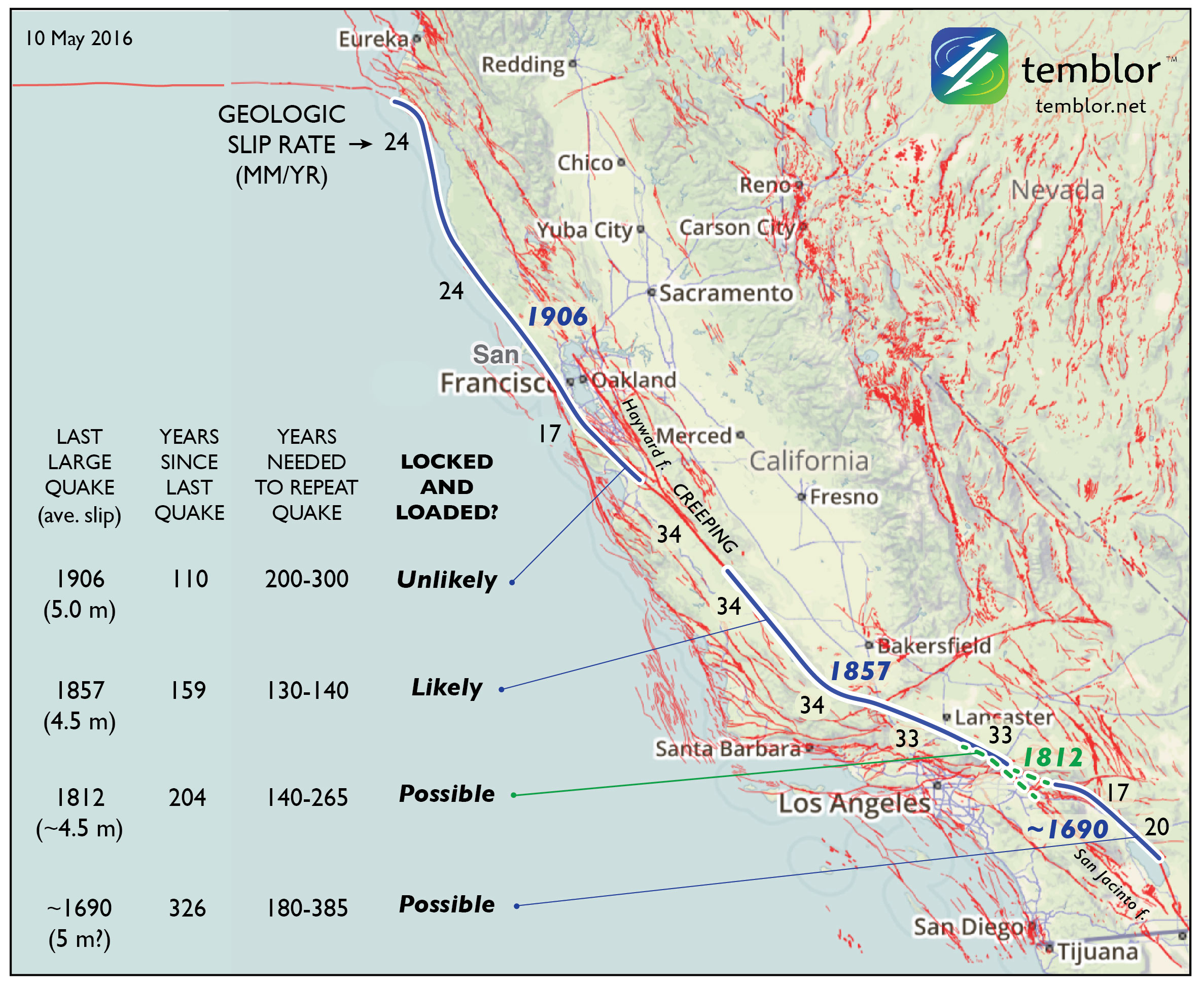
Because many misaligned, discontinuous, and bent faults accommodate the broad North America-Pacific plate boundary, the slip rate of the San Andreas is generally about half of the plate rate. Where the San Andreas is isolated and parallel to the plate motion, its slip rate is about 2/3 the plate rate, or 34 mm/yr, but where there are nearby parallel faults, such as the Hayward fault in the Bay Area or the San Jacinto in SoCal, its rate drops to about 1/3 the plate rate, or 17 mm/yr. This means that the time needed to store enough stress to trigger the next quake should not—and perhaps cannot—be uniform. So, here’s how things look to me:
The San Andreas (blue) is only the most prominent element of the 350 km (200 mi) wide plate boundary. Because ruptures do not repeat—either in their slip or their inter-event time—it’s essential to emphasize that these assessments are crude. Further, the uncertainties shown here reflect only the variation in slip rate along the fault. The rates are from Parsons et al. (2014), the 1857 and 1906 average slip are from Sieh (1978) and Song et al. (2008) respectively. The 1812 slip is a model by Lozos (2016), and the 1690 slip is simply a default estimate.
So, how about ‘locked, generally loaded, with some sections perhaps ready to go’
When I repeat Tom’s assessment in the accompanying map and table, I get a more nuanced answer. Even though the time since the last great quake along the southernmost San Andreas is longest, the slip rate there is lowest, and so this section may or may not have accumulated sufficient stress to rupture. And if it were ready to go, why didn’t it rupture in 2010, when the surface waves of the Mw=7.2 El Major-Cucapah quake just across the Mexican border enveloped and jostled that section? The strongest case can be made for a large quakeoverlapping the site of the Great 1857 Mw=7.8 Ft. Teton quake, largely because of the uniformly high San Andreas slip rate there. But this section undergoes a 40° bend (near the ‘1857’ in the map), which means that the stresses cannot be everywhere optimally aligned for failure: it is “locked” not just by friction but by geometry.
A reality check from Turkey
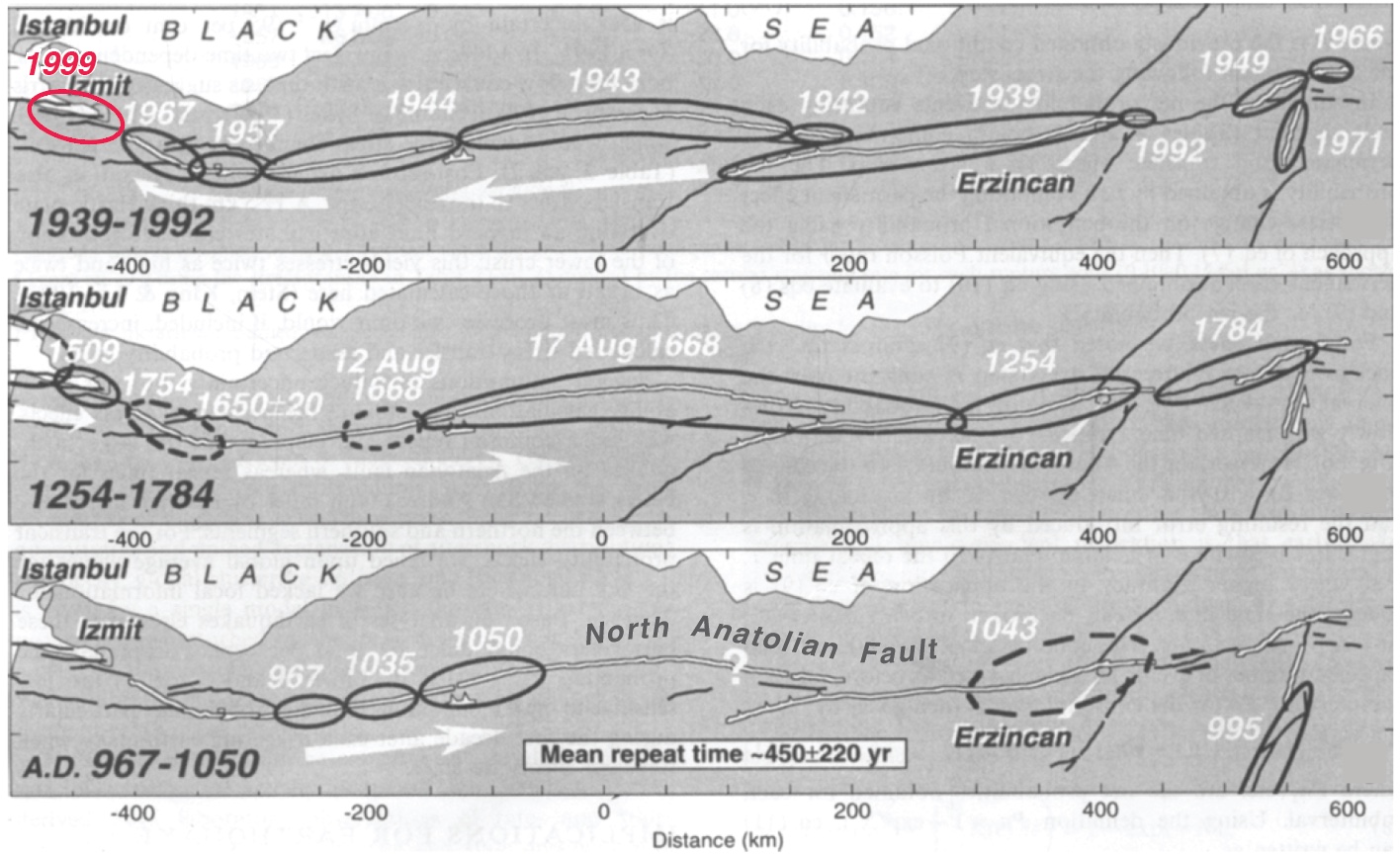
Sometimes simplicity is a tantalizing mirage, so it’s useful to look at the San Andreas’ twin sister in Turkey: the North Anatolian fault. Both right-lateral faults have about the same slip rate, length, straightness, and range of quake sizes; they both even have a creeping section near their midpoint. But the masterful work of Nicolas Ambraseys, who devoured contemporary historical accounts along the spice and trade routes of Anatolia to glean the record of great quakes (Nick could read 14 languages!) affords us a much longer look than we have of the San Andreas.
The idea that the duration of the open interval can foretell what will happen next loses its luster on the North Anatolian fault because it’s inter-event times, as well as the quake sizes and locations, are so variable. If this 50% variability applied to the San Andreas, no sections could be fairly described as ‘overdue’ today. Tom did not use this term, but others have. We should, then, reserve ‘overdue’ for an open interval more than twice the expected inter-event time.
This figure of North Anatolian fault quakes is from Stein et al. (1997), updated for the 1999 Mw=7.6 Izmit quake, with the white arrows giving the direction of cascading quakes. Even though 1939-1999 saw nearly the entire 1,000 km long fault rupture in a largely western falling-domino sequence, the earlier record is quite different. When we examined the inter-event times (the time between quakes at each point along the fault), we found it to be 450±220 years. Not only was the variation great—50% of the time between quakes—but the propagation direction was also variable.
However, another San Andreas look-alike, the Alpine Fault in New Zealand, has a record of more regular earthquakes, with an inter-event variability of 33% for the past 24 prehistoric quakes (Berryman et al., 2012). But the Alpine fault is straighter and more isolated than the San Andreas and North Anatolian faults, and so earthquakes on adjacent faults do not add or subtract stress from it. And even though the 31 mm/yr slip rate on the southern Alpine Fault is similar to the San Andreas, the mean inter-event time on the Alpine is longer than any of the San Andreas’ open intervals: 330 years. So, while it’s fascinating that there is a ‘metronome fault’ out there, the Alpine is probably not a good guidepost for the San Andreas.
If Tom’s slide is too simple, and mine is too equivocal, what’s the right answer?
I believe the best available answer is furnished by the latest California rupture model, UCERF3. Rather than looking only at the four San Andreas events, the team created hundreds of thousands of physically plausible ruptures on all 2,000 or so known faults. They found that the mean time between Mw≥7.7 shocks in California is about 106 years (they report an annual frequency of 9.4 x 10^-3 in Table 13 of Field et al., 2014; Mw=7.7 is about the size of the 1906 quake; 1857 was probably a Mw=7.8, and 1812 was probably Mw=7.5). In fact, this 106-year interval might even be the origin of Tom’s ‘once per century’ expectation since he is a UCERF3 author.
But these large events need not strike on the San Andreas, let alone on specific San Andreas sections, and there are a dozen faults capable of firing off quakes of this size in the state. While the probability is higher on the San Andreas than off, in 1872 we had a Mw=7.5-7.7 on the Owen’s Valley fault (Beanland and Clark, 1994). In the 200 years of historic records, the state has experienced up to three Mw≥7.7 events, in southern (1857) and eastern (1872), and northern (1906) California. This rate is consistent with, or perhaps even a little higher than, the long-term model average.
So, what’s the message
While the southern San Andreas is a likely candidate for the next great quake, ‘overdue’ would be over-reach, and there are many other fault sections that could rupture. But since the mean time between Mw≥7.7 California shocks is about 106 years, and we are 110 years downstream from the last one, we should all be prepared—even if we cannot be forewarned.
Sarah Beanland and Malcolm M. Clark (1994), The Owens Valley fault zone, eastern California, and surface faulting associated with the 1872 earthquake, U.S. Geol. Surv. Bulletin 1982, 29 p.
Kelvin R. Berryman, Ursula A. Cochran, Kate J. Clark, Glenn P. Biasi, Robert M. Langridge, Pilar Villamor (2012), Major Earthquakes Occur Regularly on an Isolated Plate Boundary Fault, Science, 336, 1690-1693, DOI: 10.1126/science.1218959
James H. Dietrich and Keith Richards-Dinger (2010), Earthquake recurrence in simulated fault systems, Pure Appl. Geophysics, 167, 1087-1104, DOI: 10.1007/s00024-010-0094-0.
Edward H. (Ned) Field, R. J. Arrowsmith, G. P. Biasi, P. Bird, T. E. Dawson, K. R., Felzer, D. D. Jackson, J. M. Johnson, T. H. Jordan, C. Madden, et al.(2014). Uniform California earthquake rupture forecast, version 3 (UCERF3)—The time-independent model, Bull. Seismol. Soc. Am.104, 1122–1180, doi: 10.1785/0120130164.
Robert Graves, Thomas H. Jordan, Scott Callaghan, Ewa Deelman, Edward Field, Gideon Juve, Carl Kesselman, Philip Maechling, Gaurang Mehta, Kevin Milner, David Okaya, Patrick Small, Karan Vahi (2011), CyberShake: A Physics-Based Seismic Hazard Model for Southern California, Pure Appl. Geophysics, 168, 367-381, DOI: 10.1007/s00024-010-0161-6.
Julian C. Lozos (2016), A case for historical joint rupture of the San Andreas and San Jacinto faults, Science Advances, 2, doi: 10.1126/sciadv.1500621.
Tom Parsons, K. M. Johnson, P. Bird, J.M. Bormann, T.E. Dawson, E.H. Field, W.C. Hammond, T.A. Herring, R. McCarey, Z.-K. Shen, W.R. Thatcher, R.J. Weldon II, and Y. Zeng, Appendix C—Deformation models for UCERF3, USGS Open-File Rep. 2013–1165, 66 pp.
Seok Goo Song, Gregory C. Beroza and Paul Segall (2008), A Unified Source Model for the 1906 San Francisco Earthquake, Bull. Seismol. Soc. Amer., 98, 823-831, doi: 10.1785/0120060402
Kerry E. Sieh (1978), Slip along the San Andreas fault associated with the great 1857 earthquake, Bull. Seismol. Soc. Am.,68, 1421-1448.
Ross S. Stein, Aykut A. Barka, and James H. Dieterich (1997), Progressive failure on the North Anatolian fault since 1939 by earthquake stress triggering, Geophys. J. Int., 128, 594-604, 1997, 10.1111/j.1365-246X.1997.tb05321.x
Some contractors and framers have large hands, which can pose a challenge for them when they’re trying to install the holdown nuts used to attach our Strong-Wall® SB (SWSB) Shearwall product to the foundation. Couple that challenge with the fact that anchorage attachment can only be achieved from the edges of the SWSB panel, and variable site-built framing conditions can limit access depending upon the installation sequence. To alleviate anchorage accessibility issues, we’ve required a gap between the existing adjacent framing and SWSB panel equal to the width of a 2x stud to provide access so the holdown nut can be tightened. Even so, try telling a framer an inch and a half is plenty of room in which to install the nut!Continue Reading
This week’s post was written by Kevin Gobble of Habitat for Humanity. Kevin is the Program Manager for Habitat for Humanity’s new Habitat Strong initiative. Kevin has spent over 22 years in residential construction building energy-efficient, high-performing home, and has consulted with several sustainable building programs on ways to develop their own best practices. As a third-generation builder, he has knowledge in the field of residential building science and has furthered his education to include many industry certifications — NARI Certified Remodeler, NAHB Certified Green Professional, RESNET Certified Green Rater, BPI Building Analyst, FORTIFIED evaluator, and Level 1 Infrared Thermography — while working directly with industry partners to focus on cost-effective construction solutions. Kevin has built and remodeled numerous homes to high-performance standards as certified by various building programs, including his latest project for himself: converting a condemned historic property in Atlanta to EarthCraft House Platinum.
In a previous blog post, we discussed the background of the Habitat Strong program. Habitat Strong promotes the building of resilient homes that are better equipped to withstand natural disasters in every region of the country. This program uses IBHS FORTIFIED Home™ standards and works well within Habitat’s model of building affordable, volunteer-friendly homes.Continue Reading
Larger beams are often built up out of smaller 2x or 1¾” members. This can be done for several different reasons: for the convenience of handling smaller members on the jobsite, or because solid 4x, 6x or glulam material is not readily available, or for reasons of cost. Engineered wood such as laminated veneer lumber (LVL) is often used for its high load capacity and multiple 1¾” plies are built up to get the required capacity for the application.
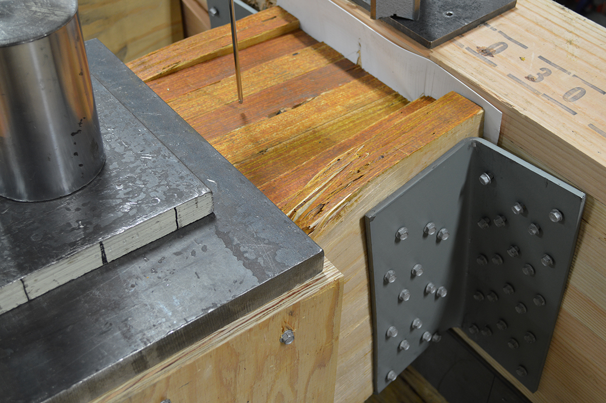
8-Ply LVL Beam in HHGU14 Test
When a built-up beam is loaded concentrically as in the test setup shown, fastening the members is not critical since that giant steel plate will load each ply of the beam. In the field, built-up beams or girders commonly support joists or beams framing into their side. The built-up members must be connected to transfer load from the loaded ply into the other plies.
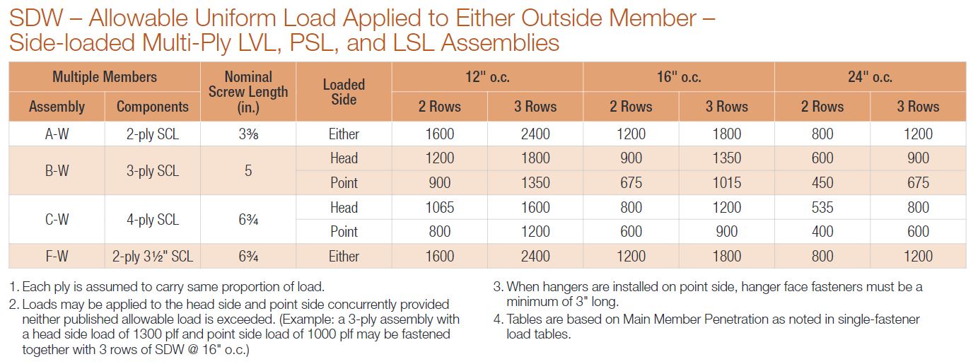
Allowable Uniform Loads and Spacing Requirements
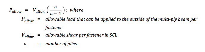
Page 303 of our Fastening Systems catalog, C-F-14 provides allowable uniform load tables for side-loaded multi-ply assemblies using LVL, PSL or LSL material. The calculation for the allowable load applied to the outside ply of a multi-ply beam is:
While uniform loads are very common, Designers often request additional information to design multi-ply beam connections to transfer concentrated loads. Simpson Strong-Tie has created a new engineering letter, L-F-SDWMLTPLY16, which complements the information in the Fastening Systems catalog by providing allowable loads in a single fastener format. Designers can use the information to calculate the number of fasteners required for a given point load.
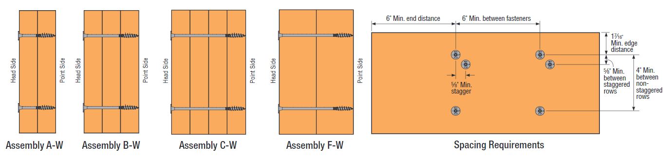
Simpson Strong-Tie® Strong-Drive® SDW EWP-Ply Screw – Allowable Loads for Side-Loaded Multi-Ply Assemblies per Screw
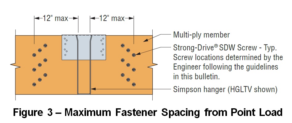
In order to ensure load transfer, the SDW screws need to be located relatively close to the connection. At first glance, it may appear challenging to fit enough fasteners while meeting the non-staggered row-spacing requirements. However, we have found that most loads can be managed by taking advantage of the ⅝” stagger allowance.
SDW – Maximum Fastener Spacing from Point Load
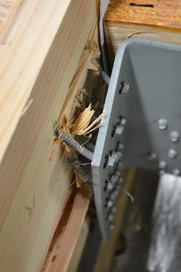
If you are curious what happened in that HHGU14 test, the screws pulled out of the header with a load slightly exceeding 101,000 pounds. Failure photo 2 shows a close-up of the pullout failure. The tested load was very close to the maximum calculated capacity for the SDS screws in the connector, so it was a great test result. What are your thoughts? Let us know in the comments below.
Who likes red rust? No one I know! How do we avoid corroding of fasteners? Corrosion can be controlled or eliminated by providing a corrosion-resistant base metal or a protective finish or coating that is capable of withstanding the exposure environment. When fasteners get corroded, they not only look bad from outside but can also lose their load capacity. To ensure continued fastener performance, we have to control for corrosion. This blog focuses on evaluating the corrosion resistance of the fasteners.
What does the building code specify?
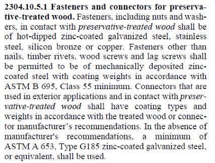
For use in preservative-treated wood, the IBC-2015 specifies fasteners that are hot-dipped galvanized, stainless steel, silicon bronze or copper. Section 2304.10.5.1 of IBC-2015 (Figure 1) covers fastener and connector requirements for preservative-treated wood (chemically treated wood). While chemically treated wood is part of the corrosion hazard, it is not the whole corrosion hazard. Weather exposure, airborne chemicals and other environmental conditions contribute to the corrosion hazard for metal hardware. In addition, the main issue with the code-referenced requirements for fasteners and connectors used with preservative-treated wood is that not all preservative treatments deliver the same corrosion hazard and not all fasteners can be hot-dip galvanized.
Figure 1: Section 2304.10.5.1 IBC-2015.
What if we want to use an alternative base material or coating for fasteners?
How do we evaluate the corrosion resistance of the alternative material or coating? The codes do not provide test methods to evaluate alternate materials and coatings. However, the International Code Council–Evaluation Service (ICC-ES) developed acceptance criteria to evaluate alternative coatings that are not code recognized for use in different environments. The purpose of acceptance criteria ICC-ES AC257, Acceptance Criteria for Corrosion-Resistant Fasteners and Evaluation of Corrosion Effects of Wood Treatment Chemicals, is twofold: (1) to establish requirements for evaluating the corrosion resistance of fasteners that are exposed to wood-treatment chemicals, weather and salt corrosion in coastal areas; and (2) to evaluate the corrosion effects of wood-treatment chemicals. In this blog post, we will concentrate on the evaluation of corrosion resistance of fasteners. The criteria provide a protocol to evaluate the corrosion resistance of fasteners where hot-dip galvanized fasteners serve as a performance benchmark. The fasteners evaluated by these criteria are nails or screws that are exposed directly to wood-treatment chemicals and that may be exposed to one or more corrosion accelerators like high humidity, elevated temperatures, high moisture or salt exposure.
The fasteners may be evaluated for any of the four exposure conditions:
Exposure Condition 1 with high humidity. This test can be used to evaluate fasteners that could be exposed to high humidity. Typical applications that fall under this category are treated wood in dry-use applications.
Exposure Condition 2 with untreated wood and salt water. This test can be used to evaluate fasteners that are above ground but exposed to coastal salt exposure.
Exposure Condition 3 with chemically treated wood and moisture. This test covers all the general construction applications.
Exposure Condition 4 with chemically treated wood and salt water. Typical applications include coastal construction applications.
Depending on the exposure condition being used for fastener evaluation, the fasteners are installed in wood that could be either chemically treated or untreated. Then the wood and the fasteners are placed in the chamber and artificially exposed to the evaluation environment. Two types of test procedures are to be completed for exposure condition 2 through 4. The purpose of these tests is not to predict the corrosion resistance of the coatings being evaluated, but to compare them to fasteners with the benchmark coating (ASTM A153, Class D) in side-by-side exposure to the accelerated corrosion environment.
ASTM B117 Continuous Salt-Spray Test
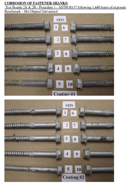
ASTM B117 is a continuous salt-spray test. For Exposure Condition 3, distilled water is used instead of salt water. The fasteners are continuously exposed to either moisture or salt spray in this test, and the test is run for about 1,440 hours after which the fasteners are evaluated for corrosion. This is an accelerated corrosion test that exposes the fasteners to a corrosive attack so the corrosion resistance of the coatings can be compared to a benchmark coating (hot-dip galvanized).
ASTM G85, Annex A5
The second test is ASTM G85, Annex A5 which is a cyclic test with alternate wet and dry cycles. The cycles are 1-hour dry-off and 1-hour fog alternatively. This is a cyclic accelerated corrosion test and relates more closely to real long-term exposure. This test is more representative of the actual environment than the continuous salt-spray test. As in the ASTM B117 test, the fasteners along with the wood are exposed to 1,440 hours, after which the corrosion on the fasteners is evaluated and compared to fasteners with the benchmark coating.
Test Method and Evaluation
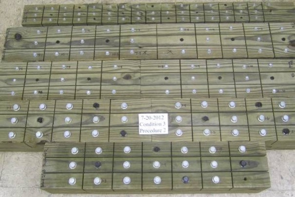
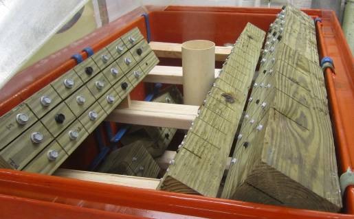
The test process involves installing 10 benchmark fasteners along with 10 fasteners for each alternative coating being evaluated. The fasteners are arranged in the wood with a spacing of 12 times the fastener diameter between the fasteners. A kerf cut is provided in the wood between the fasteners to isolate the fasteners as shown in Figure 2 and to ensure elevated moisture content in the wood surrounding the fastener shank. The moisture and retention levels of the wood are measured, and the fasteners are then installed in the chamber as shown in Figure 3 and exposed to the designated condition. The test is run for the period specified, after which the fasteners are removed, cleaned and compared to the benchmark for corrosion evaluation. Figure 4 shows the wood and fastener heads after 1,440 hours (60 days). The heads and shanks of the fasteners are visually graded for corrosion in accordance with ASTM D610. If the alternate coating performs equivalent to or better than the benchmark coating — that is, if the corrosion is no greater than in the benchmark — then the coating has passed the test and can be used as an alternative to the code-approved coating. Figure 5 shows the benchmark and alternative fasteners that are removed from the chamber after 1,440 hours.
As you can see, the alternative coatings have to go through extended and rigorous testing and evaluation as part of the approval process before being specified for any of the fasteners. Some alternative coatings provide even better corrosion resistance than the code recognized options. Sometimes, also, the thickness of these alternative coatings may be smaller than the thick coating required for hot-dip galvanized parts. Some of our coatings, such as the Double-Barrier coating, the Quik Guard® coating and the ASTM B695 Class 55 Mechanically Galvanized have gone through this rigorous testing and have been approved for use in preservative-treated wood in the AC257 Exposure Conditions 1 and 3. In addition, these coatings have been qualified for use with chemical retentions that are typical of AWPA Use Category 4A – General Ground Contact. No salt is found in AC257 Exposure Conditions 1 and 3. Please refer to our Fastener Systems Catalog, C-F-14, pages 13–15 for corrosion recommendations and pages 16–17 for additional information on coatings.
What do you look for specifically in a fastener? Do you have a preference for a certain coating type or color? Let us know in the comments below!
Figure 2: Fasteners with different coatings along with the benchmark, installed in wood and separated by kerf cuts.Figure 3: Fasteners and wood pieces installed in the chamber.Figure 4: Snap shot of fasteners in ASTM B117 chamber after 1,440 hours.Figure 5: Fasteners after 1,440 hours of exposure, removed from the wood, cleaned and compared to benchmark. Coating 1 – Benchmark (Hot- dip Galvanized) and Coating 2 (Alternative coating).
Did you know that Simpson Strong-Tie is celebrating its 60th birthday this year? We started out with one punch press and the ability to bend light-gauge steel. Then, one Sunday evening in the summer of 1956, Barclay Simpson’s doorbell rang and a request for our first joist hanger led us into the wood connector business. Since then, we’ve continued to grow that business by focusing on our engineering, research and development efforts. Some might say that nowadays we’re an engineering company that also happens to manufacture products, as evidenced by our focus on developing technology tools over the past few years such as web calculators, an updated website and design software. Our focus on technology, however, is really another aspect of our continued commitment to excellence in manufacturing and our application of the tenets of lean manufacturing.
Many of you may already be familiar with the idea of lean manufacturing made famous by Toyota in the early 2000s, along with the principles of continual improvement and respect for people. The concept of continual improvement is based on the idea that you can always make small changes to improve your processes and products. Although they were established in a manufacturing setting, these ideals ring very true for engineering as well; eliminate steps in your design process that don’t add any value to the final project and always be on the lookout for tools or techniques that can speed up your process. Thinking lean isn’t about cutting corners to get your result faster, it’s about mindfully getting rid of the steps that aren’t helping you and finding better ways of doing everyday tasks.
As structural engineers, we can find ourselves working on a variety of projects that lead us to perform repetitive calculations to check different conditions, such as varying parapet heights on the exterior of a building, or we may find ourselves working with an unfamiliar material, such as light-gauge or cold-formed steel (CFS), where we have to take some time away from design to review reference materials such as AISI S200-12 North American Standard for Cold-Formed Steel Framing. Wouldn’t it be great if there were a design tool that could help you complete your light-gauge projects more quickly, in complete compliance with current building codes?
It turns out that Simpson Strong-Tie offers a design tool called CFS Designer™ to help structural engineers improve their project design flow. This program gives engineers the ability to design light-gauge stud and track members with complex beam loading and span conditions according to building code specifications. What does that actually mean, though? Allow me to illustrate with an example of a design project.
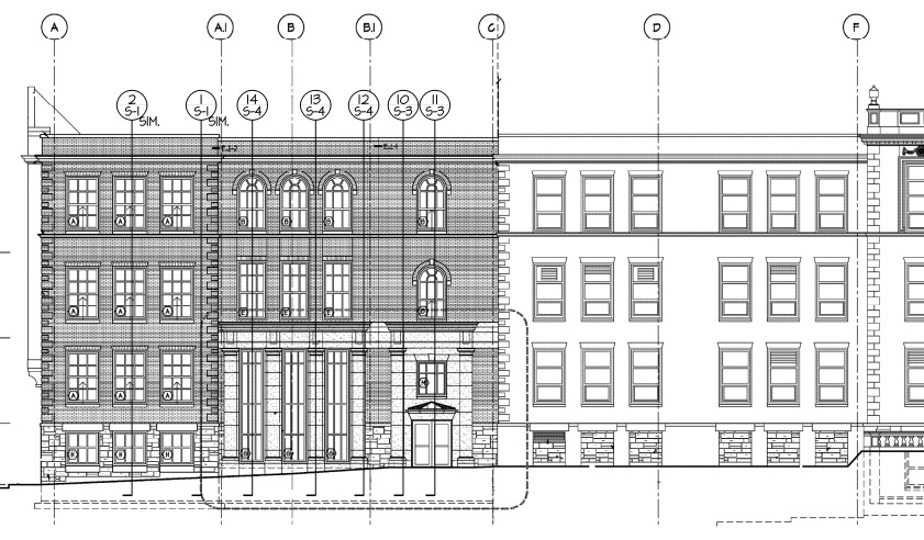
Let’s say you’re designing a building and part of your scope is the exterior wall framing, or “skin” of the building. You probably get sent some architectural plans that look something like this:
Figure 1. Sample building elevation with section marks.
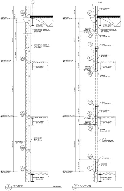
The architectural elevations will have wall section marks indicated for different framing situations. Two sample wall sections are shown in Figure 2.
Figure 2. Sample building wall sections.
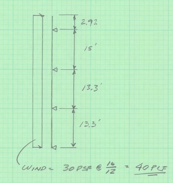
This building has several different wall section types that include door and window locations, varying parapet heights, diverse finish materials that need to meet different deflection criteria, and different connection points back to the base building. The traditional design calculation that you would need to run for one wall section might begin with a loading diagram similar to Figure 3 below.
Figure 3. Sample calculation of wall stud loading diagram.
Once you have your loading diagram generated, you would need to use reference load tables or a computer analysis program to solve for the axial and moment demands, the reactions at the pinned supports, and the member deflections.
After you determine the demand loads, you would then need to select a CFS member with sufficient properties, and you may need to iterate a few times to find a solution that meets the load and deflection parameters. After you’ve selected a member with the right width, gauge and steel strength, you’ll need to select an angle clip that can handle the demand loads, as well as fasteners to connect the clip to the CFS stud and to the base building. You would also need to also check the member design to ensure that it complies with bridging or bracing requirements per AISI. Then, after all that, you’d have to repeat the process again for all of the wall section types for your project.
Figure 4. Hmm, CFS design would sure be a lot easier if buildings were just huge windowless boxes…
Just writing out that whole process took some time, and you can imagine that actually running the calculations takes quite a bit longer. I think we can all agree that the design process we’ve outlined is time-consuming, and here’s where using CFS Designer™ to streamline your design process can really help.
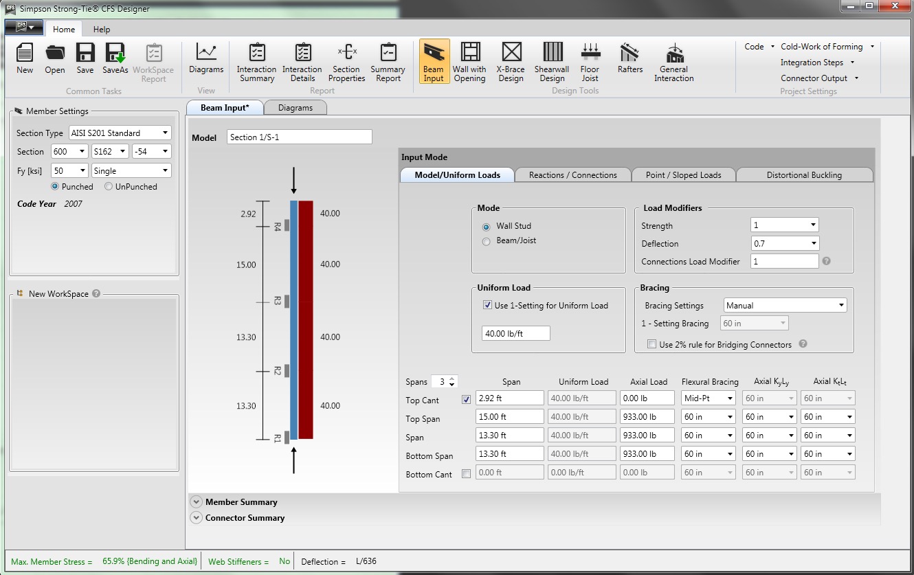
CFS Designer is a structural engineering design program that can automate many of the manual steps that are required in the design process. It has an easy-to-understand graphical user interface that allows you to input your project parameters within a variety of design modules from walls and beams, jambs and headers, X-brace walls, shearwalls, floor joists, and roof rafters. The program also enables the design of single stud or track members, built-up box-sections, back-to-back sections, and nested stud or track sections. Figure 5 shows an example of how you would input the same stud we looked at before into the program.
Figure 5. CFS Designer™ user interface for wall stud design.
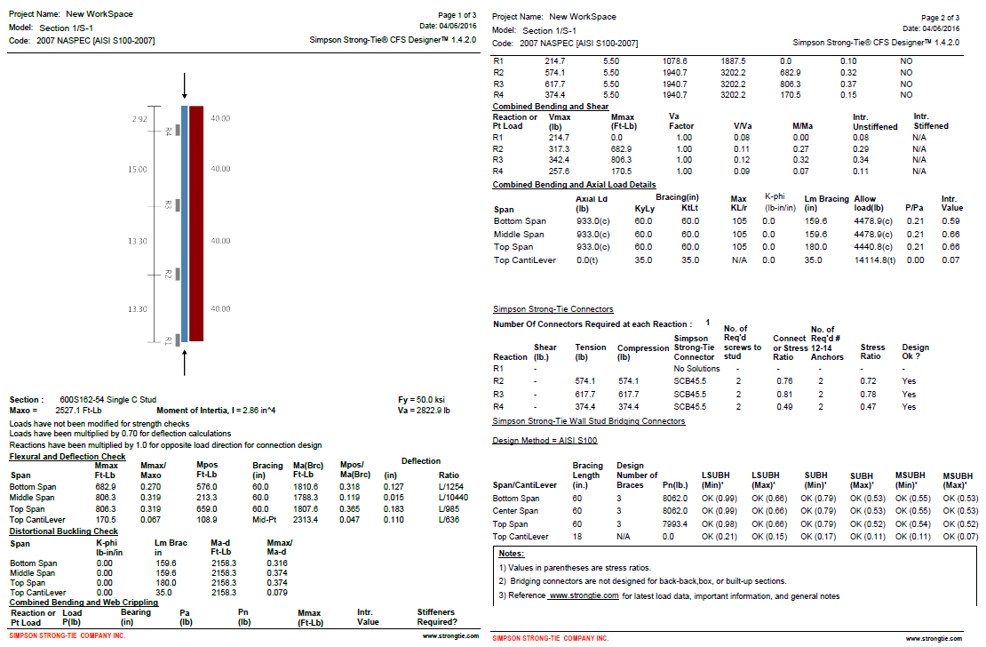
The program will generate the loading diagrams and complete calculation package for all of these different situations. And along with checking the member properties and deflection limits, CFS Designer will also check bridging and bracing requirements and provide connector solutions for the studs using tested and code-listed Simpson Strong-Tie products. Figure 6 shows an example of the summary output you would receive.
Figure 6. The comprehensive summary output page that covers the complete member design down to the bracing and connection solutions.
One unique part of the output is toward the center of the second page, under the heading “Simpson Strong-Tie Connectors.” This section summarizes the tension and compression loads at each reaction point and then shows a connector solution (such as the SCB45.5) along with the number of screws to the stud and the number of #12 sheet-metal screws to anchor back to the base building. Simpson Strong-Tie has developed and tested a full array of connectors specifically for CFS curtain-wall construction as well as for interior tenant improvement framing, which allows designers to select a connection clip straight out of a catalog without needing to calculate their own designs per the code. It’s just another way we’re helping you to get a little leaner!
The last part of the output shown in Figure 6 is titled “Simpson Strong-Tie Wall Stud Bridging Connectors.” It checks the bridging and bracing requirements per AISI S100 and selects a SUBH bridging connector, an innovative bridging solution developed by Simpson Strong-Tie that snaps into place and achieves design loads while only requiring one #10 screw to connect for 75% of applications.
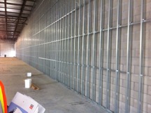
Figure 8. A close-up of the SUBH installed (left) and a wall of studs with bridging installed using the LSUBH clips (right).
You can download a free trial of CFS Designer™ and give it a test drive to see how much time it can save you on a design project. The trial version has almost full functionality, with the exception of not being able to print the output sheets. You can see purchasing information online, and you should always feel free to contact your local Simpson Strong-Tie engineering department with any questions you may have. I hope you are able to take advantage of this great tool to further improve your everyday design processes. We will be sure to keep you updated on our latest technology tools that help speed up the design process. If you’re using CFS Designer, we’d like to hear your thoughts about the program. Please share them in the comments below.
“Structures are connections held together by members” (Hardy Cross)
I heard this quote recently during a presentation at the Midwest Wood Solutions Fair. I had to write it down for future reference because of course, all of us here at Simpson Strong-Tie are pretty passionate about connections. I figured it wouldn’t take too long before I’d find an opportunity to use it. So when I started to write this blog post about the proper selection of a truss-to-wall connection, I knew I had found my opportunity – how fitting this quote is!
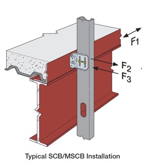
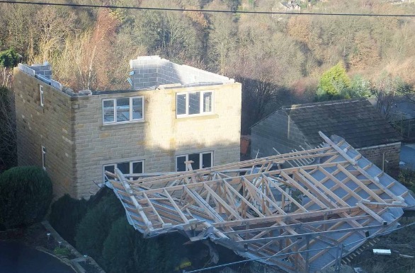
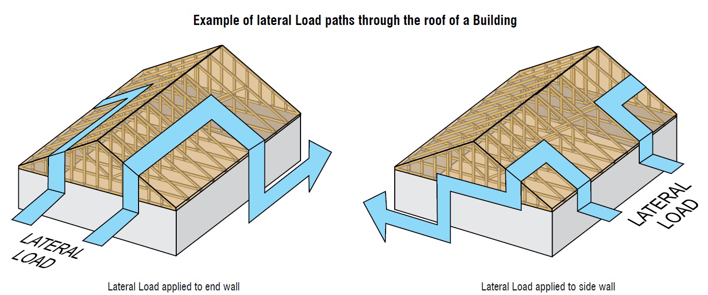
There are plenty of photos of damage wrought by past hurricanes to prove that the connection between the roof and the structure is a critical detail. In a previous blog post, I wrote about whose responsibility it is to specify a truss-to-wall connection (hint: it’s not the truss Designer’s). This blog post is going to focus on the proper specification of a truss-to-wall connection, the methods for evaluating those connections under combined loading and a little background on those methods (i.e., the fun stuff for engineers).
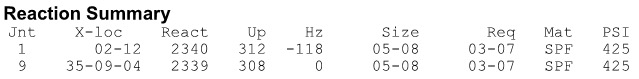
Take a quick look at a truss design drawing, and you will see a reaction summary that specifies the downward reaction, uplift and a horizontal reaction (if applicable) at each bearing location. Some people are tempted to look only at the uplift reaction, go to a catalog or web app, and find the lowest-cost hurricane tie with a capacity that meets or barely exceeds the uplift reaction.
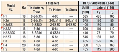
However, if uplift was the only loading that needed to be resisted by a hurricane tie, why would we publish all those F1 and F2 allowable loads in our catalog?
Of course, many of you know that those F1 and F2 allowable loads are used to resist the lateral loads acting on the end and side walls of the building, which are in addition to the uplift forces. Therefore, it is not adequate to select a hurricane tie based on uplift reactions alone.
Excerpt from BCSI (2015 Version)
Where does one get the lateral loads parallel and perpendicular to the plate which must be resisted by the truss-to-wall connection? Definitely not from the truss design drawing! Unless otherwise noted, the horizontal reaction on a truss design should not be confused with a lateral reaction due to the wind acting on the walls – it is simply a horizontal reaction due to the wind load (or a drag load) being applied to the truss profile. It is also important to note that any truss-to-wall connection specified on a truss design drawing was most likely selected based on the uplift reaction alone. There may even be a note that says the connection is for “uplift only” and does not consider lateral loads. In this case, unless additional consideration is made for the lateral loads, the use of that connector alone would be inadequate.
Say, for example, that the uplift and lateral/shear load requirements for a truss-to-wall connection are as follows:
Uplift = 795 lb.
Shear (parallel-to-wall) = 185 lb. (F1)
Lateral (perp-to-wall) = 135 lb. (F2)
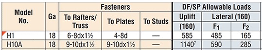
Based on those demand loads, will an H10A work?
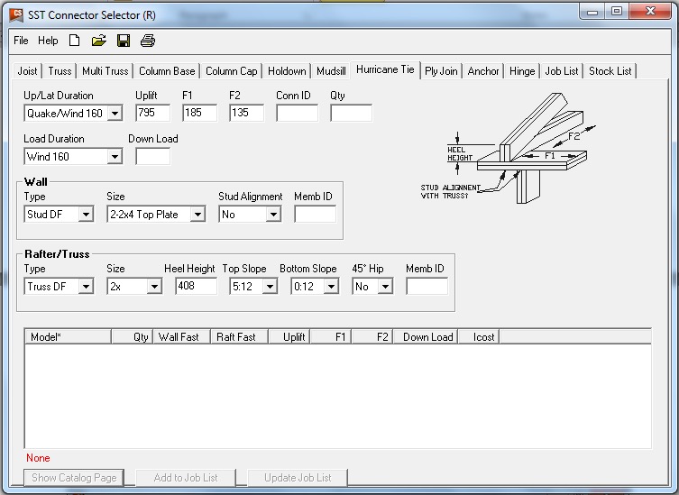
An initial look at the H10A’s allowable loads suggests it might be adequate. However, when these loads are entered into the Connector-Selector, no H10A solution is found.
Combined Uplift, F1 and F2 Loads
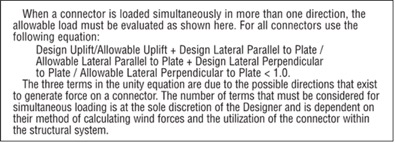
Why? Because Connector-Selector is evaluating the connector for simultaneous loading in more than one direction using a traditional linear interaction equation approach as specified in our catalog:
If the shear and lateral forces were to be resisted by another means, such that the H10A only had to resist the 795 lb. of uplift, then it would be an adequate connector for the job. For example, the F1 load might be resisted with blocking and RBC clips, and the F2 loads might be resisted with toe-nails that are used to attach the truss to the wall prior to the installation of the H10A connectors. However, if all three loads need to be resisted by the same connector, then the H10A is not adequate according to the linear interaction equation.
Uplift Only
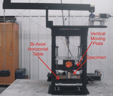
Some might question how valid this method of evaluation is – Is it necessary? Is it adequate? How do we know? And that is where the interesting information comes in. Several years ago, Simpson Strong-Tie partnered with Clemson University on an experimental study with the following primary objectives:
1. To verify the perceived notion that the capacity of the connector is reduced when loaded in more than one direction and that the linear interaction equation is conservative in acknowledging this combined load effect.
2. To propose an alternative, more efficient method if possible.
Three types of metal connectors were selected for this study – the H2.5A, H10, and the META20 strap – based on their different characteristics and ability to represent general classes of connectors. The connectors were subjected to uni-axial, bi-axial and tri-axial loads and the normalized capacities of the connectors were plotted along with different interaction/design surfaces.
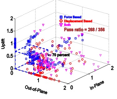
These interaction plots were used to visualize and parameterize the combined load effect on the capacity of the connectors. The three different interaction plots that were examined were the traditional linear relationship, a quadratic interaction surface and a cuboid design space.
Tri-axial Test FrameInteraction plot for tri-axial loads on a cuboid design space
The results? Not only was the use of the linear interaction equation justified by this study, but a new, more efficient cuboid design surface was also identified. It provides twice the usable design space of the surface currently used for tri-axial loading and still provides for a safe design (and for the bi-axial case, it is even more conservative than the linear equation). This alternative method is given in our catalog as follows:
Now we can go back to the H10A and re-evaluate it using this alternative method:
As it turns out, the H10A does have adequate capacity to resist the simultaneous uplift, shear and lateral loads in this example. This just goes to show that the alternative method is definitely worth utilizing, whenever possible, especially when a connector fails the linear equation.
For more information about the study, see Evaluation of Three Typical Roof Framing-to-Top Plate/Concrete Simpson Strong-Tie Metal Connectors under Combined Loading.
What is your preferred method for resisting the combined shear, lateral and uplift forces acting on the truss-to-wall connections? Let us know in the comments below!
We’re partnering with folks at Fine Homebuilding on a video series on how to build a deck that is code compliant and that highlights the critical connections of a deck. This series is called Ultimate Deck Build 2016. The video series comprises five videos that walk professionals through the recent code changes for the key connections of a deck.
The series features David Finkenbinder, P.E., a branch engineer for Simpson Strong-Tie who is passionate about deck codes and safety. He offers information on load resistance and the hardware that professionals can use at the crucial connections to make a deck code compliant. “This was a great opportunity to collaborate with the team at Fine Homebuilding, to communicate the connections on a typical residential deck and the role that they serve to develop a strong deck structure,” said David. “These same connections would also likely be common in similar details created by an Engineer, when designing a deck per the International Building Code (IBC).”
The videos are being released every Wednesday during the month of March and feature the following deck connections:
Ledger Connection: This is the primary connection between a deck and a house. David tells the Fine Homebuilding team about various code- compliant options for attaching a deck ledger to a home.
Beam and Support Posts: David explains how connectors at this critical point can prevent uplift and resist lateral and downward forces. He also discusses footing sizes and post-installation anchor solutions.
Joists: This video reviews proper joist hanger installation and the benefits of installing hurricane ties between the joists and the beams. David goes into common joist hanger misinstallations, such as using the wrong fasteners or using a joist hanger at the end of a ledger.
Guardrail Posts: David reviews the different ways that you can attach a guardrail post so as to resist an outward horizontal load.
Stairs: David explains code-compliant options for attaching stringers to a deck frame.
Make sure to watch the series and let us know what you think. For more information, Fine Homebuilding has created an article titled “Critical Deck Connections.”
(Please note: this article is member-only/subscription content, so to read it you’ll need to either subscribe online or pick up the April/May issue of Fine Homebuilding.)
We use cookies on this site to enhance your user experience. By clicking "I AGREE" below, you are giving your consent for us to set cookies. Privacy PolicyI AGREE
Privacy & Cookies Policy
Privacy Overview
This website uses cookies to improve your experience while you navigate through the website. Out of these cookies, the cookies that are categorized as necessary are stored on your browser as they are essential for the working of basic functionalities...
Necessary cookies are absolutely essential for the website to function properly. This category only includes cookies that ensures basic functionalities and security features of the website. These cookies do not store any personal information.
Any cookies that may not be particularly necessary for the website to function and is used specifically to collect user personal data via analytics, ads, other embedded contents are termed as non-necessary cookies. It is mandatory to procure user consent prior to running these cookies on your website.


 next generation of super-computers—because the current generation
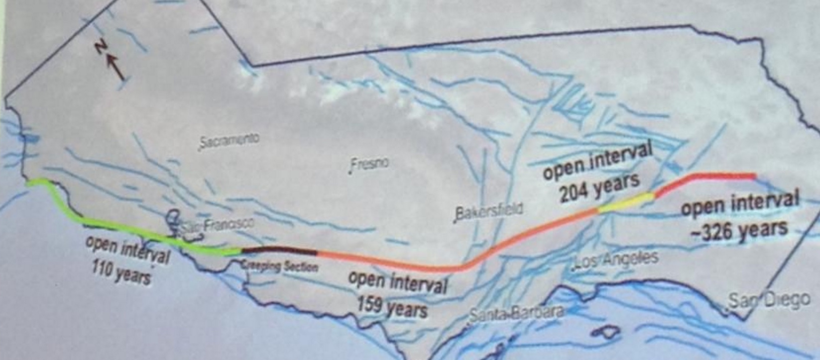
 overlapping the site of the Great 1857 Mw=7.8 Ft. Teton quake, largely because of the uniformly high San Andreas slip rate there. But this section undergoes a 40° bend (near the ‘1857’ in the map), which means that the stresses cannot be everywhere optimally aligned for failure: it is “locked” not just by friction but by geometry.